The odd story so far

In the previous post, we took a tour through various formulations of probability – mainly by exploring the notion of odds, which captures exactly the same idea as probability, but using different numbers – a probability of one half, like of getting a head on the toss of a coin, corresponds to an odds of one. A probability, by definition, is a number between 0 (not gonna happen) and 1 (a sure thing), but the statistician’s odds of a particular outcome of a process, or ‘trial’, can be any number bigger than 0 – with no upper limit. Here, the odds of an outcome is the ratio of

1. the probability of the particular outcome, to
2. the total probability of all the other outcomes,

The fact that the values are open ended, without upper limit, is one of the features of the formulation of statistics in terms of odds that makes it attractive for some computational applications. That’s because sometimes there is extra unnecessary complexity involved in making sure that formulas don’t take on values greater than 1 – but there really is no intellectual content added by talking about odds instead of probabilities.

Although these alternative formulations in terms of probability, statistician’s odds, and betting odds can take some getting used to, there is no real controversy here.

Exercise to consolidate material from the previous post:

In the opening track of Jeff Wayne’s Musical version of [H.G. Wells’s] The War of the Worlds, we hear:

“The chances of anything coming from Mars, are a million to one,” he [Ogilvy the Astronomer] said     

(AaaaaaaaaaH    aaaaaaah)

“The chances of anything coming from Mars, are a million to one,”

but still, they come!

Question: He said “chances”. Discuss. A model answer, including several bonus components, to follow in a later post.

What is the Likelihood?

I have often been told that “a likelihood is not a probability”. Well, odds are not, at face value, probabilities, but they encode probabilities in a way that is very specific and precisely defined. Likelihoods, on the other hand, are in fact just probabilities – even the numbers are the same. We don’t even have to do any arithmetic to find corresponding values of probabilities and odds that encode the same idea.

Probability Likelihood Chance – Three words, one meaning.

What is the Likelihood FOR?

There are many ways of solving mathematical problems – including statistical problems. In any particular field of study, one can learn a modest number of very useful approaches that one keeps coming back to, but there are always different ways of unpacking a puzzle. Usually, we check complicated calculations precisely by finding at least two quite different ways of getting to the same answer.

However, in all the activities that come under the umbrella ‘statistical estimation’, it is hard to think of a single concept that is as pervasive and important as what we usually mean when we say ‘likelihood’ instead of probability. If you want to feel comfortable talking about statistics, you’re going to want to know how to use the formal term ‘likelihood’ in a sentence.

A classic problem in statistics is something like this:

We ‘randomly’ sampled 100 people. Of these, 14 turned out to be left handed. What is our best estimate of the proportion of people who are left handed, and, crucially, how ‘good’ is our estimate?

Most of us would guess that the best estimate is that 14% of people are left handed, because that’s what we observed in our sample – and we (let’s say, in this case) have no reason to believe that our sampling technique was ‘biased’ towards finding either left or right handed people. We believe every person in the population had the same chance of being sampled. Maybe we put everyone’s name on a piece of paper and tossed them all around in a great hat before blindly picking 100 bits of paper.

On the other hand, we should be surprised if the proportion of left handed people in the population were precisely 14 percent. It could easily be 13% or 15%, and frankly, it is unlikely to be an exact whole number – maybe it’s 14,321%! Who knows.

So we want to develop useful terminology, and good analYsis, to define and quantify what we mean by the ‘inherent uncertainty’ in a statistically based estimate. We want to have a general method, or formula, for handling questions of this nature; We don’t just want to address the question about left handedness, or just analyse the particular data set consisting of 100 observations, of which 14 are of one type (left handed) while the other 86 are not of this type. (In this case, the ‘others’ are all the same, namely right handed – but we might be estimating the proportion of people who have the desirable blood type O negative, rather than any one of several other types.)

We want to come up with a coherent approach to a class of problems of this type, namely:

• estimating the proportions of subgroups in some ‘underlying population’, given
• observations on some ‘random’ sample,

The only game in town is investigation of this thing called ‘the likelihood’. In fact, analysis of ‘the likelihood’ is almost the only game in town for many other kinds of stats related questions.

Statistical Experiments / Trials

Back to basics:

If I toss a ‘fair’ coin, the probability of getting a head is the same as the probability of getting a tail – namely one half.

Another perfectly normal, and equally correct, way of saying this is:

If I toss a ‘fair’ coin, the likelihood of getting a head is the same as the likelihood of getting a tail – namely one half.

It would take a pretty creative analyst to find a way of interpreting these two remarks through a lens which considers the meaning of likelihood to be different from the meaning of probability. They are not different.

Now what if I bend the coin, so that it has a probability of 75% (i.e. of three quarters) of landing on heads, and only a 25% probability (one quarter) of landing on tails? Although it looks a little weird, we can legitimately mix the terminology and say:

the probability of getting heads (75%) is three times the likelihood of getting tails (25%).

i.e. the odds of getting heads is three!

This conventional concept of probability, or likelihood, as it is often called in the context of assessing probabilities of ‘outcomes’ of some formally defined ‘trial’, is something we try to express very precisely – sometimes going to great lengths to do so. A likelihood function is nothing more or less than:

• a specification of the probabilities of various outcomes of a process, for which
• the rules are nominally known (and have been spelled out), but
• there is some inherent randomness (often called stochasticity).

There is nothing mysterious about the throw of a die, or the toss of a coin. We know precisely how it works. However, the outcome, in each case, depends so finely on details of how the throwing is done, that, under the usual conditions that apply to such tosses, we essentially have no control over the outcomes of specific ‘trials’ or ‘repeats’ of the process/experiment. Not only can we not guarantee a head or a tail, we can’t even make one outcome a little bit more likely than the other. I can of course gently drop a coin on a table from a height of a few millimetres in such a way that I can exert considerable control over whether it comes up heads or tails – but this is far removed from flicking a coin high in the air with the impetus of arm and thumb, and letting it fall on the ground – in which case it really is impossible to set it up to be more likely to end up one way or another.

While outcomes may be ‘random’, this does not mean that each outcome is equally likely. The probability that a randomly accosted stranger is left handed is not the same as the probability that they are right handed. In order to specify a ‘likelihood function’ we need to know the probabilities of each possible outcome:

Likelihood of result one = l₁

Likelihood of result two = l₂

.

.

Likelihood of result N = l_N

We should check that once all possible results (i=1, …N) have been enumerated, the proposed probabilities l_i add up to one. This captures the point that each time we perform the trial, one of the listed possible results is bound to emerge. The coin will come to rest with either the head or the tail facing up. In a sensibly constructed model world, where we can hope to calculate interesting things, there will be no other options, like the coin landing on an edge, or in a vat of boiling lava.

Sometimes we don’t use a discrete list to enumerate all possible outcomes of a trial. The result of the experiment of trying to measure the length of some lizard’s body, with a ruler, might be a number that lies between 0 and 300mm – and not all results will be equally likely. In such cases we represent the likelihoods of various results with a ‘distribution’.

So there are ‘discrete’ and ‘continuous’ versions of ‘likelihood construction‘, by which we mean:

• listing all possible results of a stochastic experiment, or ‘trial’, and

• assigning each of them its likelihood,

There are many interesting and challenging technical details along the way. Most people do not need to fret over these details – but it’s useful to understand, viscerally, that figuring out the details of ‘the likelihood’ is just about the central recurring theme of statistical analysis.

Sampling

When we survey people, for instance to see what proportion of them are left handed, we try to do so in such a way that each individual has the same chance of being chosen. We might want to know the proportion of women tennis players, registered with the WTA, that are left handed. In this case it’s not a good idea to pick people at random from those who make it into grand slam finals – because this is a subgroup that is heavily biased in favour of the top ten players, and even within this group, heavily and unevenly biased in favour of the top two or three. Depending on the year in which this survey is planned, you would be exposed to various biases, depending, for example, on whether a famous left hander or a famous right hander was in good form. A standard way to ‘obtain a sample’ would be to make a list of all the players in question, and then find a way of picking some of them by a process which gives each one the same chance of being chosen.

But if there’s a database with all the players details, why do we not check whether the database also contains the information on handedness – then we can know, precisely, for example, that 127 of the 984 players registered with the tour are left handed. That would indeed be the way to answer this particular question. However, for the really interesting or genuinely important questions of this kind, sampling is the only way to get the information we need, because it’s simply not feasible to get all the relevant data on each relevant person.

The trouble with sampling is that it’s seldom possible to give every person the same chance of being chosen. We have to find imperfect ways of making it at least reasonably balanced, so that the sample we obtain is ‘sufficiently representative’ of the population which we want to investigate. The challenges of sampling are real, and no sensible researcher ignores them, but for our present needs, getting deeper into this now would be a distraction, rather than a deepening of the analysis.

All conventional statistical reasoning, like all other mathematical modelling endeavours, leans heavily on thinking about idealised situations – Model Worlds – in which things are simpler than in the real world. Without this, we would drown in distracting details long before we’ve learned anything worth knowing. When we have spelled out the idealised rules and/or facts, like declaring that

• 10 percent of professional women tennis players are left handed, and that
• we can construct samples in which every tennis player has the same chance of being selected

then we can use some clever mathematics to answer questions like:

• If we randomly choose 10 players, what is the likelihood that precisely 1 of them will be left handed?
• If we randomly choose 20 players, what is the likelihood that none of them will be left handed?
• If we randomly choose 100 players, what is the likelihood that the number of left handed players chosen is between 10 and 20? (being careful to be clear whether we mean to include or exclude the ‘limiting’ or ‘edge’ cases of 10 and 20)

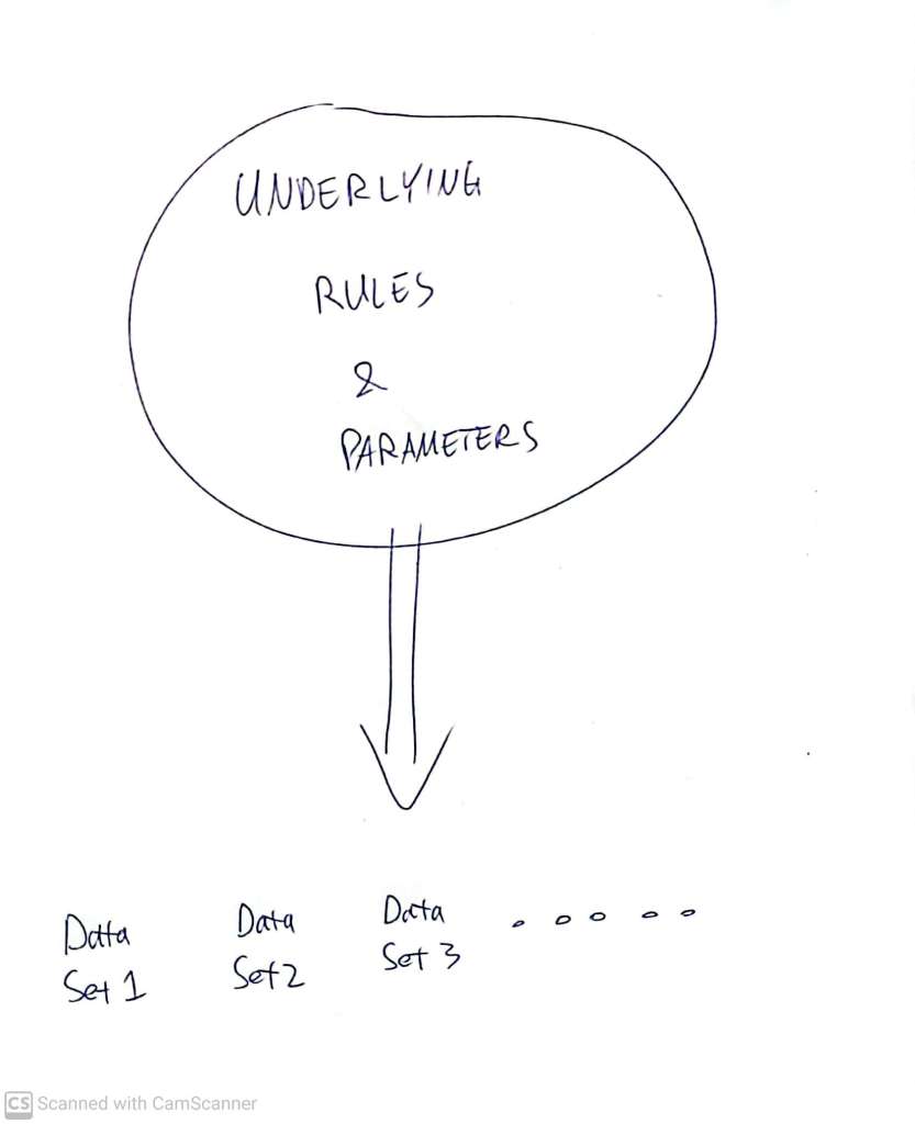
Note the pattern: the likelihood discourse hinges on spelling out

• some underlying fundamental rule which drives the randomness in the experiment, and
• exactly how likely all the possible outcomes of some experiment are.

Sometimes there is considerable complexity between the underlying driving rule and the details of the sampling (even if it is totally unbiased). This is the heart and soul of likelihood function/distribution analysis

For example – if 10% of individuals in some group are left handed, then we know that a randomly chosen one has a likelihood of 10% (a probability of 0.1) of being left handed. If we sample three people, we could end up with either 0, 1, 2 or 3 left handers, and it requires some careful thought to derive a formula which expresses the likelihood of each of these cases. Dealing with this categorical/count based sampling (as opposed to measurement based sampling – like investigating the heights of the players, for example) is what the famous Binomial Distribution was invented for.

Fortunately, for all sorts of generic situations which keep coming up, someone has done the ‘heavy lifting’ and figured out how to derive the appropriate likelihood functions. We can sometimes just use them as they are described in the literature, or we can adapt them as appropriate to our particular situation.  

The big inversion

There is a very particular difficulty – likelihood theory is a well developed way for understanding the probabilities of getting one or other result, IF we know some very specific crucial details of an underlying system and process:

But – this is not really the situation in which we usually find ourselves. More usually, we are planning, or have done, an experiment, and we want to milk the data for knowledge about what the underlying rules are – which is pretty much the inverse!

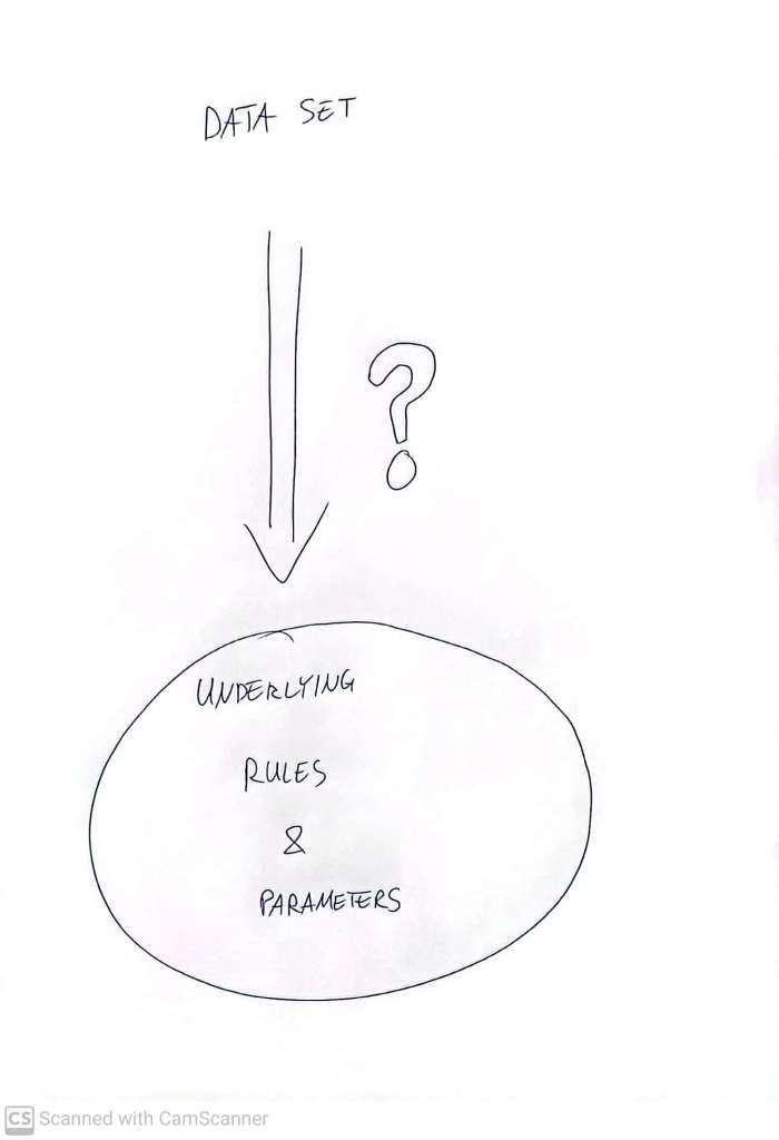
The real magic of statistical experiments, and the analysis of the data they produce, lies in the sensible ‘inversion’ of this logic of the likelihood. When we do an experiment to understand a system, we are interested in asking questions broadly of this form:

Given the experimental outcomes which we have observed – what can we know about the process?

It is tempting to ask things like:

Given that 10 out of 100 tennis players surveyed were found to be left handed, what is the probability that precisely 10 percent of players are left handed?

while being careful not to muddy the waters by saying

Given that 10 out of 100 tennis players surveyed were found to be left handed, what is the likelihood that precisely 10 percent of players are left handed?

This line of questioning takes us straight into the heart of statistical philosophy, but right now we are mainly interested in more prosaic technical details. For example, if the population of formally registered professional women’s tennis players is 1074 (or any other number that is not a multiple of ten) then it’s simply not possible to have precisely ten percent of them be left handed. This little problem we can handle by not being fixated on precise particular values, and by talking instead about ranges of values:

Given that 10 out of 100 tennis players surveyed were found to be left handed, what is the probability that the actual fraction of left handed players lies between 9.0 and 11.0 percent?

Now we’ve sidestepped the problem of talking about a particular value with infinite precision. The more serious niggle is that this is what mathematicians call an ill-posed problem. The way we have just tossed out this question leaves certain details unspecified – and depending on how we fill in these details, we can get different perfectly correct answers.

Imagine you’ve interviewed two people, one of whom turned out to be lefthanded. You probably already knew that the proportion of left handed people is NOT between 45% and 55%. According to some generic formula, which exists free from prior knowledge of the subject matter, there may be an implicit view that 50% is not obviously wrong – but you know it’s wrong.

It’s asking too much of an equation/formula to have ‘prior’ subject matter knowledge about the real world, so we have to choose our words carefully when talking about inference i.e. when trying to ‘invert’ the logic of the likelihood.

Bayesian Analysis

There is a simple but brilliantly conceived, and very rich, core set of ideas called ‘Bayesian analysis’, which sensibly,  works with ‘prior’ and ‘posterior’ information/estimates – estimates which apply prior to, and after, we get data from a particular experiment.

Once you have spelled out the ‘prior’ information/estimate, you need to define the experiment you are conducting, and derive the applicable likelihood function which we’ve been talking about. The central theorem of Bayesian analysis explains how to combine the

• the prior,
• the likelihood, and
• the data

into a ‘posterior’ estimate. Usually, the prior and posterior versions of information are spelled out through probability distributions, which capture the probability that some or other value, or range of values, is the answer to our fundamental question – like the proportion of people who have blood type O negative.

An excellent standard demonstration of this Bayesian process concerns a diagnostic test. Imagine we have engineered a very cheap new genetic test with which we can determine whether someone has a particular risk factor for severe disease during SARS-CoV-2 infection. The test is not perfect, but it gives the ‘true’ answer (as discernable via some expensive ‘gold standard’ test) 99% of the time. More precisely:

• It has a 99% chance of getting the right result when the risk factor is present – which is sometimes framed as ‘the test has a 99% sensitivity.
• and it has a 99% chance of getting the right result when the risk factor is absent – which is sometimes framed as ‘the test has a 99% specificity.

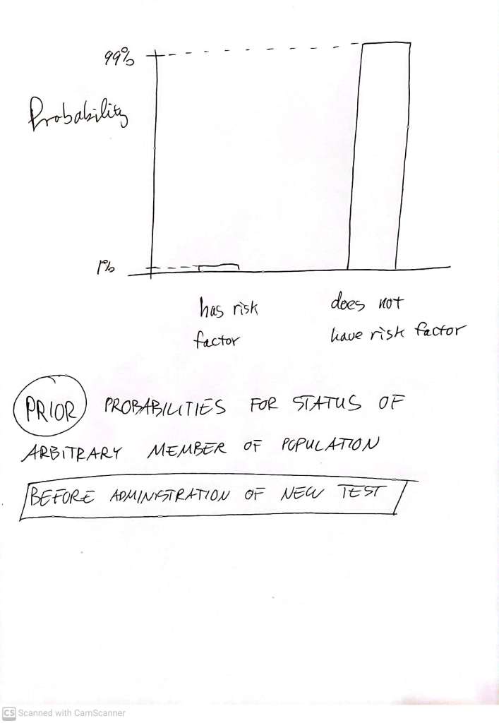
Now assume that we know, from detailed studies, that almost exactly 1 percent of people have this genetic risk factor, and we want to use this cheap new test to see, in various contexts, who these particular people are, to ensure that they get appropriate treatment. We have a drug which is specifically effective in combating complications from the particular risk factor – but is useless against Covid complications arising for other reasons, and has potentially serious side effects. This drug should therefore not be be given to patients unless we are pretty sure that they have the particular genetic risk factor, even if they have already developed severe covid.

If we just pick any person from the population, by some process which gives every individual an equal chance of being chosen, and we test the sampled person, and the cheap test says this person has the risk factor – how likely is it that this person in fact has the genetic risk factor we are looking for?

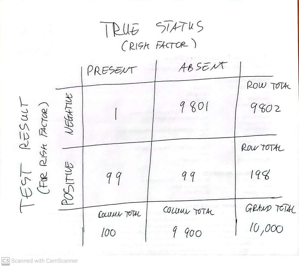
Imagine screening 10,000 people with this test. If 1% of them have the genetic risk factor for severe SARS-CoV-2 disease, that’s 100 of the people in our screened cohort. Of these, we expect to correctly identify 99, and to miss 1. Among the 9,900 who don’t have the risk factor, we expect to correctly infer, for 99% of them (9801 of them) that they don’t have it, and we expect to incorrectly flag 1% of them (99 of them) as having it.

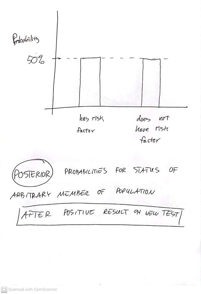
If all we know is that someone got a ‘positive’ test result (test claims they have the risk factor) then all we know is that they are one of the 198 people, among the 10,000 screened, who got a positive result. But of the 198 who get positive results, 99 are ‘true’ positives, and the other 99 are ‘false’ positives. Reread the previous paragraph if that’s not clear. In other words, only half of these positive results are correct! Whenever the condition we are testing for is relatively rare, the ‘true positives‘ share a pool of ‘all positives’ with lots of ‘false positives’.

So, if you prescreen yourself for this condition, using the cheap test, and you get a positive result (i.e. the test claims that you have the genetic risk factor) and you take this at face value, and then, when you find yourself diagnosed with Covid, your doctor immediately prescribes the drug designed to offset the complications which the risk factor threatens to bring – then you have a very substantial chance of subjecting yourself to a futile and potentially unpleasant or even harmful treatment.

Let’s repeat the reasoning with our steps a little more aligned to the usual language of “Bayes’ Theorem“. We have the prior state of our knowledge being that 1% of people have the risk factor – so if you just pick a person from the population, giving everyone an equal chance of being chosen, then the probability of this person having the severe covid disease risk factor is 1% (Prob = 0.01):

Now we do the test – and it comes up ‘positive’ for the genetic marker. As per the above reasoning, we now have the ‘posterior’:

If that test had been negative, we would have had a posterior with a probability of 99.99% that the person is free of the risk factor, and a probability of just 0.01% (probability = 0.0001) of having the risk factor. There is no way to talk meaningfully about the posterior if you do not specify the prior – so this approach shows us how important it is to be clear about what you already know even before you do your experiment. Of course, in many situations, we don’t really know how to spell out our ‘prior’ knowledge in terms of something as fully specied as a ‘prior distribution’. We can’t always (or even very often) confidently say something like:

Even before doing my survey, I know that the proportion of left handed tennis players is a number between 10% and 20%, with anything in that range being equally probable

Not to worry – it turns out that this Bayesian framework bears up very well when we interpret the prior and posterior probability distributions in a slightly less technical way:

Even before doing my survey, I know that the proportion of left handed tennis players is a number between 10% and 20%, with anything in that range being equally plausible.

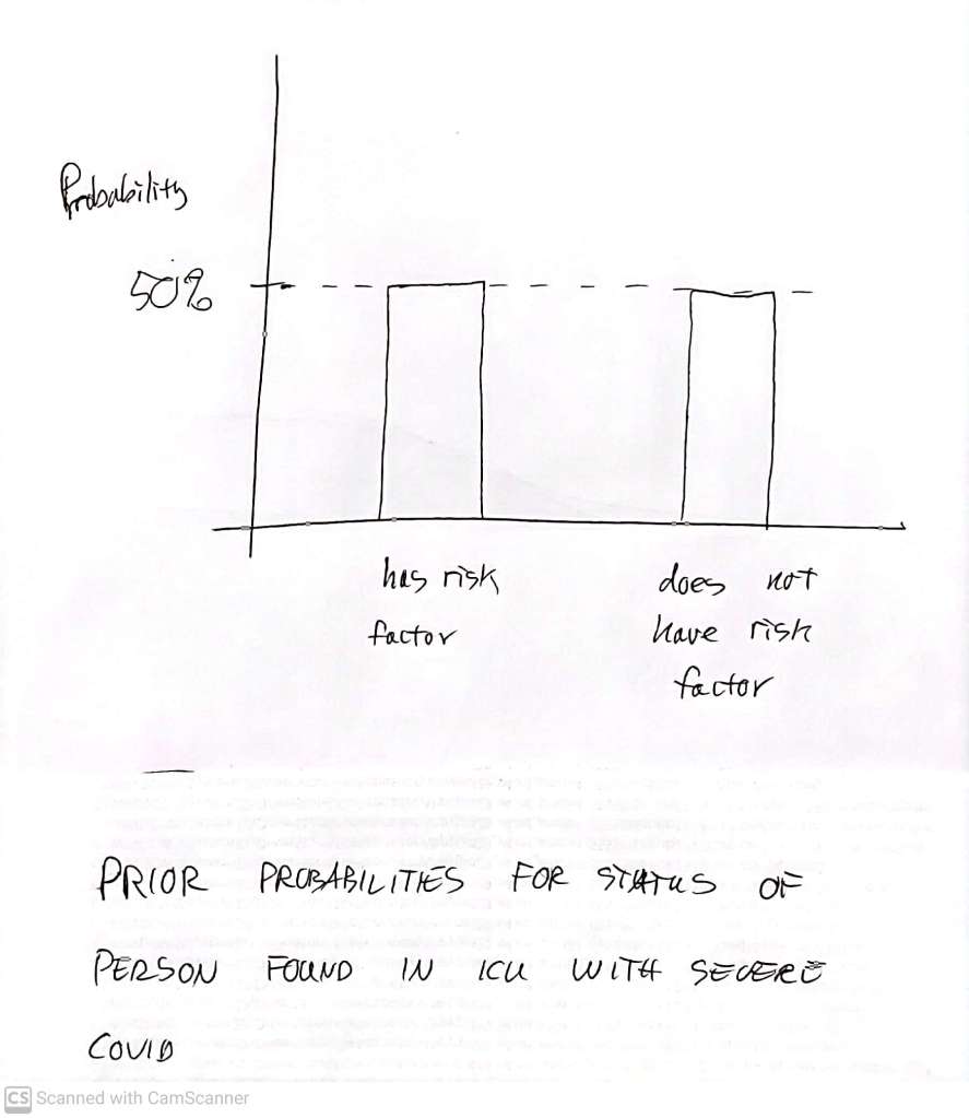
Back to identifying people at risk of severe Covid: This time, instead of picking someone at random from the population, we go to the ICU at the city hospital, and we test the patients there who are being treated for Covid. These are people who are already experiencing severe covid, or they would not be in the ICU. There will be various reasons they have severe covid – but our genetic risk factor will be one of them. Individuals with this risk factor have a better chance of getting to the ICU than people without it, so the prior distribution is no longer given by the population level breakdown. What is it then? Hard to say for sure – but we may have some idea, based on various sources. Perhaps we believe that half the people in the ICU actually have the risk factor. Then before we run the test on one of these people, the prior looks like this

If we now get a positive result, the posterior looks like this (see assignment below to get started on checking it yourself)

If we get a negative result on the patient in ICU, the posterior looks like this

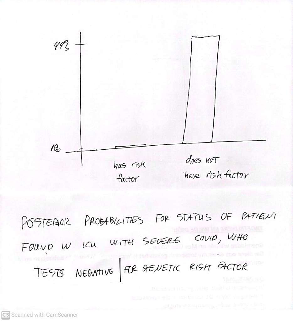
So when we start with a ‘uniform’ prior – which we did here in the ICU patients just for illustration – then the probabilities in the posterior are what we naively expect. We will return to this point – later! The important practical operational point is that by using the test closer to the point of interest, when we have already limited our group to one (the ICU patients) that is enriched for individuals with the condition we are looking for – then the true positives are no longer swamped with false negatives, and the test performs rather well, and can be safely used in making a serious clinical decision. The use of information is very context dependent – and these contextual factors come in multiple layers, affecting even in the basic assignment of probabilities of what is the case, given some data.

This use of priors and posteriors to capture ‘plausibility’ or ‘belief’ is a bit more controversial than their use to capture carefully crafted pre- and post-experiment scenarios in terms of conventional probabilities. In practice, however, this slightly less formal way of using the formulation of probability to capture confidence, or belief, is really the most common use of this Bayesian reasoning. In the real world we simply don’t have well defined ‘priors’ much of the time. Books have been written, …

Frequentist AnalYsis

There is also another fundamental way of thinking about levels of confidence and belief that you can attribute to experimental data – the so called ‘frequentist’ approach. This approach dispenses with the need to specify a prior distribution of values of whatever we are estimating. That forces us to be very carefully about what we mean by probability, and NOT to embrace the more subjective flavours which are allowed by Bayesian reasoning.

When we talk about a likelihood function, we are talking about predicting the probability of this or that happening when we execute some formal process – crucially, some formal process which we can repeat as frequently as we want. The outcome of each trial is truly not known up front, even though the exact actual properties of the process have been specified and taken into account in the likelihood calculation, which describes what we expect to see over the course of many repeats of the trial

On the other hand, when we have some data from having just done an experiment, we can no longer really talk of ‘predicting’ anything about forthcoming events. Therefore it can be considered a bit weird to say – here’s what I predict will happen when we peek in the back of the book of all knowledge to see what this or that quantity actually is (like the proportion of people who are born left-handed). There is no ‘stochastic process’ which can yield a variety of outcomes, according to some (likelihood) distribution. Whenever you peek in the back of the book of all knowledge – the answer is going to be the same.

The way to get around this conundrum, which crosses linguistic, mathematical, and philosophical domains, is to make statements not of the form

Given the data, here is the probability that the truth is thus and such

But rather:

If I did the experiment many times and analysed each data set in this particular way, then the probability of being right (in some specific sense), would be the following.

This is a mouthful and a mindful. It’s the way we formally talk when we mention things like ‘Confidence Intervals’ for estimates – and it requires a fuller discussion than we can do here, to do it justice.

Altogether now

Some pretty clever people have figured out the details of these frequentist and Bayesian ideas, so that all we need to do build the likelihood function, and then we can make sensible statements about imperfectly precise estimates of real world quantities. There are lots of details – both important and interesting.

The point is that a likelihood distribution/function is a formula of some kind which tells us how probable it is that some or other result will arise in a suitably well defined process/experiment – and the most sacred key point today is that there is no difference between a likelihood and a probability – no matter what someone says.

Postscript/Apology

The astute reader, having possibly learned some details about likelihood functions, may be left feeling cheated – because the claim was that there was some subtle reason that there is a common misconception that ‘a likelihood is not a probability’ – and these dots have certainly not been joined. Guilty as charged. But in my defence: before we can understand this little slip, we need to have some feeling for how the term ‘likelihood’ is typically used.  

Stay tuned for “A likelihood is too a probability (TWO)”

Consolidation Assignment

Work out the details of the simple diagnostic scenario described above: Fill in the blocks in the “2 by 2” (2X2) ‘Contingency table’.

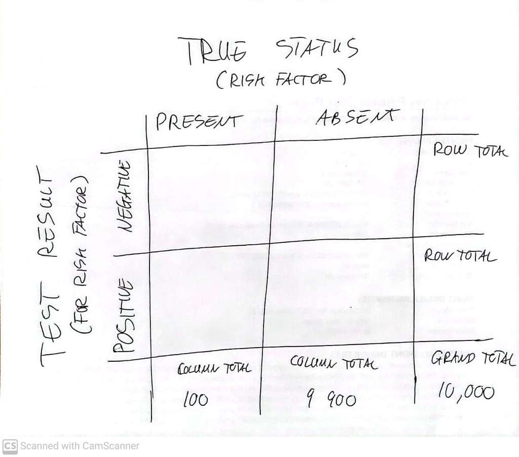
You might get something like this:

If you are worried about the arbitrary choice of screening 10,000 individuals, you can avoid choosing a ‘screened sample’ size and do the whole table in fractions/proportions of the population who (would) fall into the various boxes, if they were selected and tested. Try it yourself.

Next – redo the whole exercise but start with the ICU-based prior, and check whether the numbers given above are in factocorrect.